What a Good Fit Can Tell Us
A model can describe a pattern remarkably well while leaving the process behind it unresolved.
A machine with a slot and a chute
Think of a model as a machine with a slot and a chute. You put something into the slot; something comes out of the chute. A weather model takes measurements and returns a forecast. A model of a cell takes recorded features and returns a label or a prediction. The machine may be very complicated inside, but the basic relationship is familiar: an input is transformed into an output according to a rule.
Learning reconstructs that rule from examples. We show the machine inputs paired with answers, or ask it to predict missing pieces of a record. Then we adjust it until its answers improve. What makes the modern version remarkable is the range of things it can accept and the number of adjustable parts it can contain. What remains old is the inferential problem. From a collection of examples, what have we learned about the process that produced them?
This question matters especially when the next request differs from the examples. Recognizing a familiar pattern is one accomplishment. Predicting what will happen in an unfamiliar circumstance is another. Explaining why it will happen asks for something stronger again. These ambitions are connected, but we should not let the ease of moving between them in language conceal the evidence needed to move between them in science.
A cell as a point
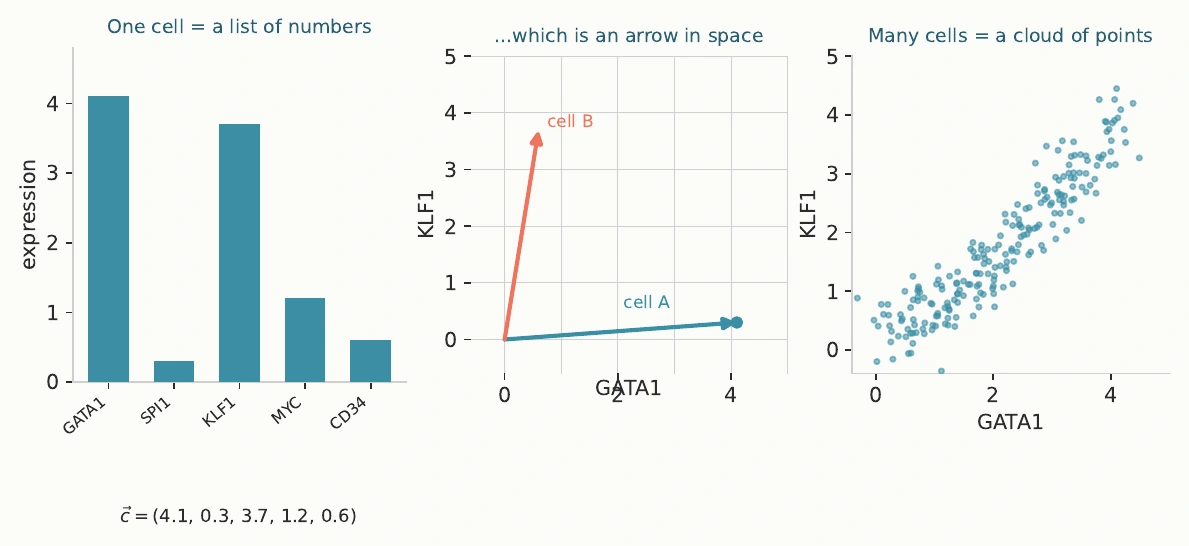
The machinery begins with an ordinary list of numbers. Imagine recording two measurements of a cell: 4.1 for one feature and 0.3 for another. The list, written as (4.1, 0.3), is a vector. Plot the first number horizontally and the second vertically, and the same list becomes a point. Draw an arrow from the origin to that point, and it becomes a direction with a length. These are different views of one object.
With thousands of measurements, we have thousands of coordinates. We cannot draw all the axes, but the arithmetic stays familiar. Adding two vectors means adding corresponding entries. Scaling a vector means multiplying every entry by the same number. A weighted combination is several vectors added together after being scaled. Nothing mysterious happens when the list becomes long; the operations simply happen on more entries.
For the model, this list is the cell as represented in the data. That qualification matters. The actual cell contains history, spatial relationships, and unmeasured states. A recorded profile contains what a particular measurement system captured. We can represent many cells as a cloud of points and study the shape of that cloud. Its structure may be informative, but the translation from cell to point has already selected what information enters the machine.
Similarity and transformations
How can a machine compare two lists? One elementary operation is the dot product: multiply corresponding entries and add the results. For (3, 1) and (2, 2.4), the answer is 3 times 2, plus 1 times 2.4, giving 8.4. Geometrically, this measures aligned length. Divide out the lengths of the vectors, and the resulting cosine similarity measures their alignment without treating a larger overall magnitude as greater agreement.
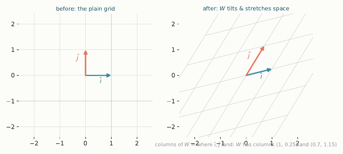
A matrix organizes many such calculations. Each row supplies a set of weights; its dot product with the input produces one output coordinate. A matrix with three rows can therefore transform a two-number input into a three-number output. In a two-dimensional picture, a linear transformation can stretch, rotate, or shear the coordinate grid. The matrix's columns tell us where the original coordinate arrows land. The rest follows from combinations of those arrows.
Doing one linear transformation after another is itself a linear transformation. A long stack of matrices can collapse into one combined matrix if nothing nonlinear sits between them. Depth alone therefore does not create the variety of shapes associated with neural networks. The crucial ingredient is the operation between the matrices: something that allows the transformation to bend, rather than merely stretch and turn, the relationships among points.
The bend that changes the problem
A simple nonlinear operation keeps positive numbers and replaces negative ones with zero. This is the rectified linear unit, usually shortened to ReLU. A neuron forms a weighted sum, adds an offset, and applies such an operation. Many neurons arranged together make a layer. Repeating layers lets the network rearrange the geometry of its input, so relationships that were difficult to separate can become easier to read.
The smallest memorable example is exclusive-or. At the corners of a square, label two opposite corners 1 and the other two 0. No single straight boundary separates the labels. A hidden layer with a nonlinear bend can transform the points so a straightforward output rule succeeds. This is a concrete gain in expressive power. It explains why a network is more than a large collection of straight-line calculations.
Yet expressive power answers a question about what can be represented, not which representation learning will recover. Approximation theorems establish possibilities under specified conditions; they do not promise that training on finite examples will discover the generating mechanism. A machine may have enough flexibility to draw the right curve and many wrong curves as well. The usefulness of the bend creates a new responsibility: finding evidence that distinguishes among the possibilities it makes available.
Attention, without mysticism
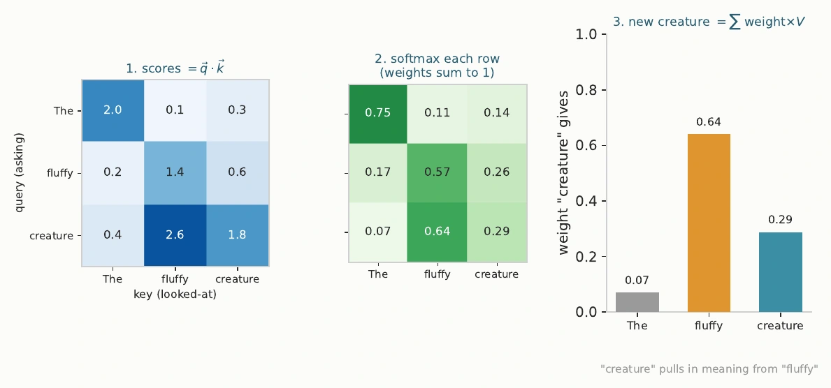
In a transformer, tokens first become learned vectors. A token might be a piece of a word or another unit chosen to represent an input. Each token's representation is then updated in relation to its context. Attention supplies one way to decide which other positions should contribute. Learned transformations create queries, keys, and values. Query–key comparisons produce scores, which are normalized into weights; the values are combined using those weights.
Suppose the scores associated with three relevant positions are 2.6, 1.8, and 0.4. Exponentiating and dividing by their total gives weights of approximately 64 percent, 29 percent, and 7 percent. The update draws most heavily from the first position. This weighted mixing can encode important relationships across an input. Its interpretation depends on the learned representations; a numerical alignment need not correspond to a single familiar human concept.
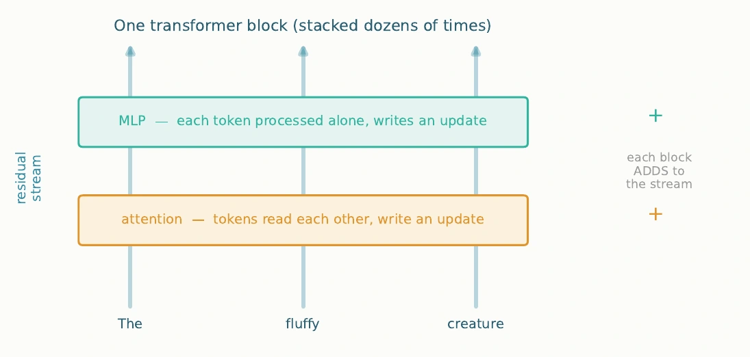
Attention and a feed-forward network add updates to a running representation, often called the residual stream. Repeating these blocks produces increasingly contextual representations. Vaswani and colleagues introduced this transformer architecture in 2017. The machinery is impressive, but it is still a sequence of specified operations applied to numerical inputs. Looking inside it helps us separate the computation a model performs from the scientific interpretation we place on its output.
What the fit leaves open
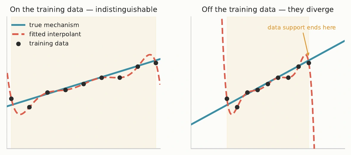
Now return to a plot with a handful of measured points. Several curves can pass through them. They may agree wherever we measured and tell different stories beyond that region. A fitted curve can fill gaps effectively without being a unique account of the process behind the observations. This is the distinction between interpolation as a predictive accomplishment and mechanism as an explanatory claim.
The distinction is not a rule that prediction is shallow or that neural networks cannot learn structure. A useful predictor may capture real relationships, and a mechanistic account may itself be approximate. What matters is the inference we make from success. Good performance under familiar conditions supports reliability under those conditions. A claim about the generating process needs tests that plausible alternatives would fail.
I want to keep that question in view as the machinery becomes larger: what has the evidence actually selected? A million adjustable parts do not answer it automatically, and neither does a billion. A model can earn a place in scientific work through accurate prediction, useful representation, or productive hypotheses. Each contribution becomes clearer when we name it precisely. The next step is to ask when the available observations can identify the explanation we hope the machine has learned.